Tablespaces
This document provides an overview of YSQL Tablespaces and demonstrates how they can be used to specify data placement for tables and indexes in the cloud.
Overview
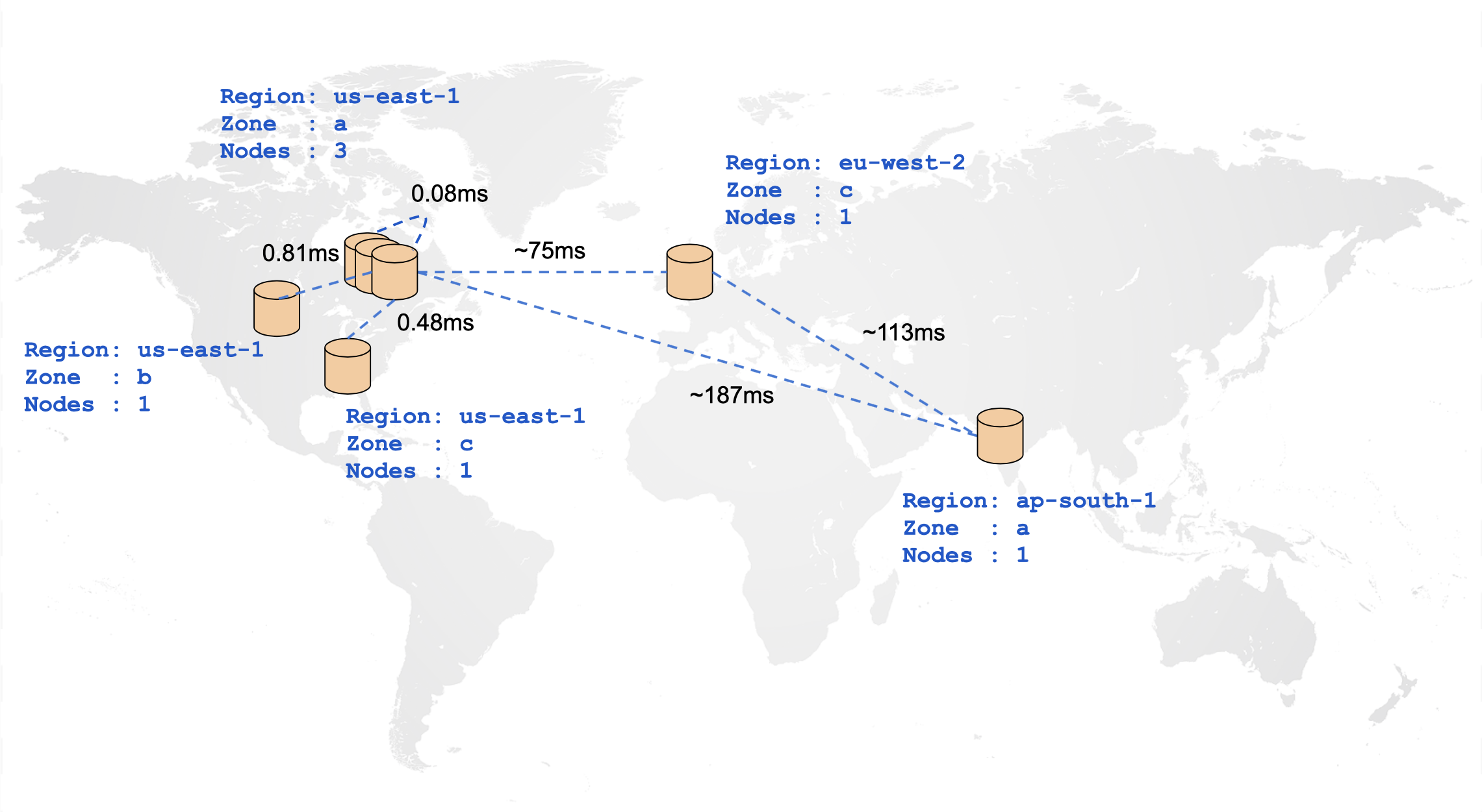
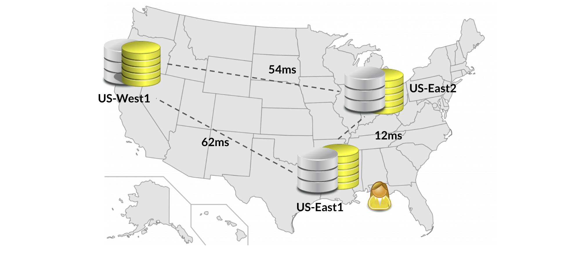
In a distributed cloud-native database such as YugabyteDB, the location of tables and indexes plays a very important role in achieving optimal performance for any workload. The following diagram illustrates the ping latencies amongst nodes in a geo-distributed cluster. It is very apparent that nodes closer to each other can communicate with visibly lesser latency than nodes physically far away from each other.
Given the impact of distance on node-to-node communication, it is highly useful to be able to specify at a table level, how its data should be spread across the cluster. This way, you can move tables closer to their clients and decide which tables actually need to be geo-distributed. This can be achieved using YSQL Tablespaces. YSQL Tablespaces are entities that can specify the number of replicas for a set of tables or indexes, and how each of these replicas should be distributed across a set of cloud, regions, zones.
This document describes how to create the following:
- A cluster that is spread across multiple regions across the world.
- Tablespaces that specify single-zone, multi-zone and multi-region placement policies.
- Tables associated with the created tablespaces.
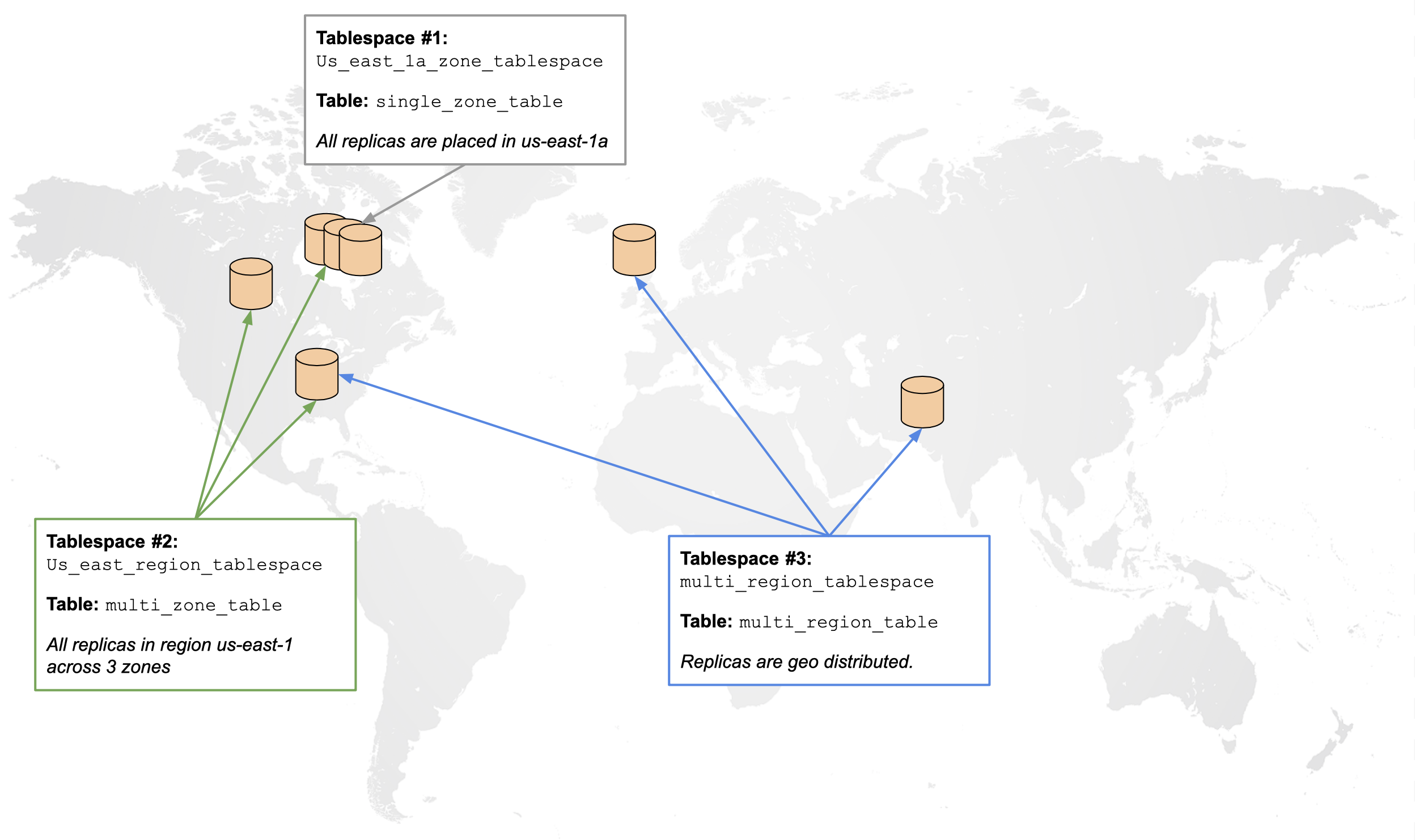
This can be summarized in the following diagram:
In addition, this document demonstrates the effect of geo-distribution on basic YSQL commands through an experiment. This experiment, outlined in the following sections, measures the effect of various geo-distribution policies on the latencies observed while running INSERTs and SELECTs. The results can be seen in the following table:
| Geo-Distribution | INSERT Latency (ms) | SELECT Latency (ms) |
|---|---|---|
| Single Zone | 4.676 | 1.880 |
| Multi Zone | 11.825 | 4.145 |
| Multi Region | 836.616 | 337.154 |
Cluster Setup
The differences between single-zone, multi-zone and multi-region configuration becomes apparent when a cluster with the following topology (as per the preceding cluster diagrams) is deployed. This topology is chosen for illustrative purposes as it can allow creation of node, zone, region fault-tolerant placement policies in the same cluster with minimum nodes.
| Region | Zone | Number of nodes |
|---|---|---|
| us-east-1 (N.Virginia) | us-east-1a | 3 |
| us-east-1 (N.Virginia) | us-east-1b | 1 |
| us-east-1 (N.Virginia) | us-east-1c | 1 |
| ap-south-1 (Mumbai) | ap-south-1a | 1 |
| eu-west-2 (London) | eu-west-2c | 1 |
Cluster creation
A cluster with the preceding configuration can be created using the following yugabyted commands:
bin/yugabyted start                            \
  --base_dir=/home/yugabyte/<IP1>/yugabyte-data      \
  --listen=<IP1>                               \
  --master_flags "placement_cloud=aws,placement_region=us-east-1,placement_zone=us-east-1a" \
  --tserver_flags "placement_cloud=aws,placement_region=us-east-1,placement_zone=us-east-1a"
bin/yugabyted start                            \
  --base_dir=/home/yugabyte/<IP2>/yugabyte-data      \
  --listen=<IP2>                               \
  --join=<IP1>                                 \
  --master_flags "placement_cloud=aws,placement_region=us-east-1,placement_zone=us-east-1b" \
  --tserver_flags "placement_cloud=aws,placement_region=us-east-1,placement_zone=us-east-1b"
bin/yugabyted start                            \
  --base_dir=/home/yugabyte/<IP3>/yugabyte-data      \
  --listen=<IP3>                               \
  --join=<IP1>                                 \
  --master_flags "placement_cloud=aws,placement_region=us-east-1,placement_zone=us-east-1c" \
  --tserver_flags "placement_cloud=aws,placement_region=us-east-1,placement_zone=us-east-1c"
bin/yugabyted start                            \
  --base_dir=/home/yugabyte/<IP4>/yugabyte-data      \
  --listen=<IP4>                               \
  --join=<IP1>                                 \
  --tserver_flags "placement_cloud=aws,placement_region=ap-south-1,placement_zone=ap-south-1a"
bin/yugabyted start                            \
  --base_dir=/home/yugabyte/<IP5>/yugabyte-data      \
  --listen=<IP5>                               \
  --join=<IP1>                                 \
  --tserver_flags "placement_cloud=aws,placement_region=eu-west-2,placement_zone=eu-west-2c"
bin/yugabyted start                            \
  --base_dir=/home/yugabyte/<IP6>/yugabyte-data      \
  --listen=<IP6>                               \
  --join=<IP1>                                 \
  --tserver_flags "placement_cloud=aws,placement_region=us-east-1,placement_zone=us-east-1a"
bin/yugabyted start                            \
  --base_dir=/home/yugabyte/<IP7>/yugabyte-data      \
  --listen=<IP7>                               \
  --join=<IP1>                                 \
  --tserver_flags "placement_cloud=aws,placement_region=us-east-1,placement_zone=us-east-1a"
The cluster can be created using YugabyteDB Anywhere Admin Console by setting the following options in the Create Universe page:

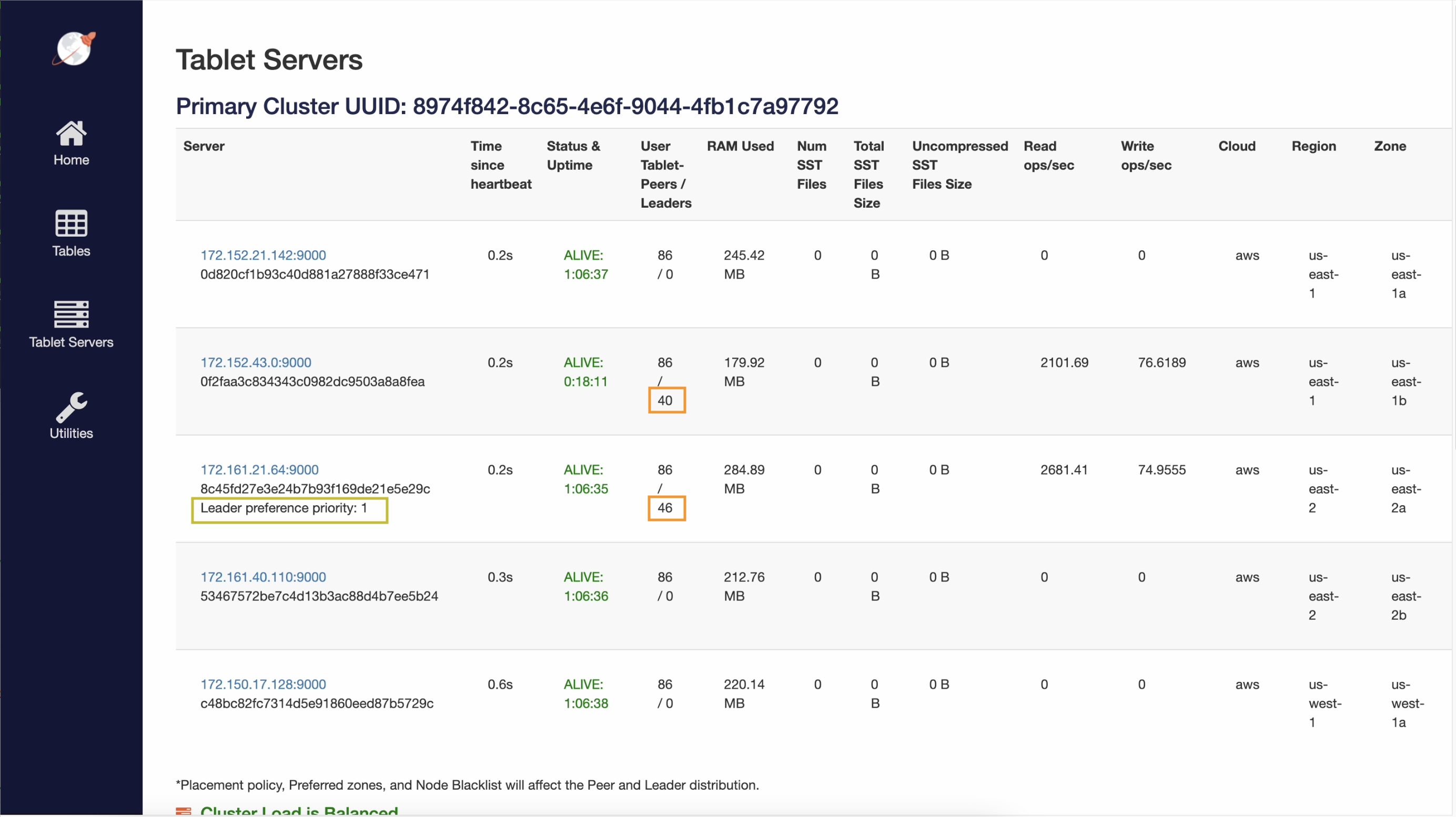
After cluster creation, verify if the nodes have been created with the given configuration by navigating to the Tablet Servers page in the YB-Master UI

Create a single-zone table
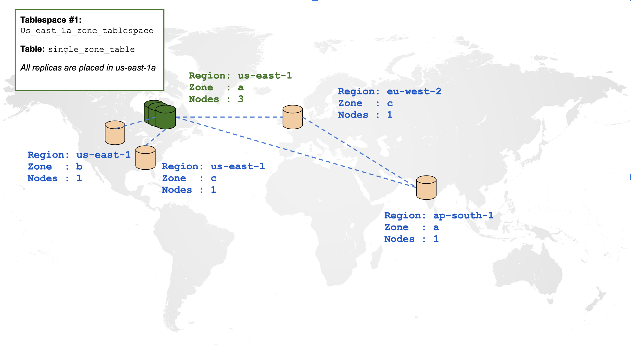
By default creating any tables in the preceding cluster will spread all of its data across all regions. By contrast, let us create a table and constrain all of its data within a single zone using tablespaces. The placement policy that we will use can be illustrated using the following diagram:
 Create a tablespace outlining the preceding placement policy and a table associated with that tablespace:
CREATE TABLESPACE us_east_1a_zone_tablespace
  WITH (replica_placement='{"num_replicas": 3, "placement_blocks": [
    {"cloud":"aws","region":"us-east-1","zone":"us-east-1a","min_num_replicas":3}]}');

CREATE TABLE single_zone_table (id INTEGER, field text)
  TABLESPACE us_east_1a_zone_tablespace SPLIT INTO 1 TABLETS;
Note from the preceding cluster configuration that the nodes in us-east-1a were 172.152.29.181, 172.152.27.126 and 172.152.22.180. By navigating to the table view in the YB-Master UI, you can verify that the tablet created for this table was indeed placed in us_east_1a_zone:

Now let us measure the latencies incurred for INSERTs and SELECTs on this table, where the client is in us-east-1a zone:
yugabyte=# INSERT INTO single_zone_table VALUES (1, 'field1'), (2, 'field2'), (3, 'field3');
Time: 4.676 ms
yugabyte=# SELECT * FROM single_zone_table;
 id | field
----+--------
  2 | field2
  1 | field1
  3 | field3
(3 rows)

Time: 1.880 ms
Create a multi-zone table
The following diagram is a graphical representation of a table that is spread across multiple zones within the same region:

CREATE TABLESPACE us_east_region_tablespace
  WITH (replica_placement='{"num_replicas": 3, "placement_blocks": [
    {"cloud":"aws","region":"us-east-1","zone":"us-east-1a","min_num_replicas":1},
    {"cloud":"aws","region":"us-east-1","zone":"us-east-1b","min_num_replicas":1},
    {"cloud":"aws","region":"us-east-1","zone":"us-east-1c","min_num_replicas":1}]}');

CREATE TABLE multi_zone_table (id INTEGER, field text)
  TABLESPACE us_east_region_tablespace SPLIT INTO 1 TABLETS;
The following demonstrates how to measure the latencies incurred for INSERTs and SELECTs on this table, where the client is in us-east-1a zone:
yugabyte=# INSERT INTO multi_zone_table VALUES (1, 'field1'), (2, 'field2'), (3, 'field3');
Time: 11.825 ms
yugabyte=# SELECT * FROM multi_zone_table;
 id | field
----+--------
  1 | field1
  3 | field3
  2 | field2
(3 rows)

Time: 4.145 ms
Create a multi-region table
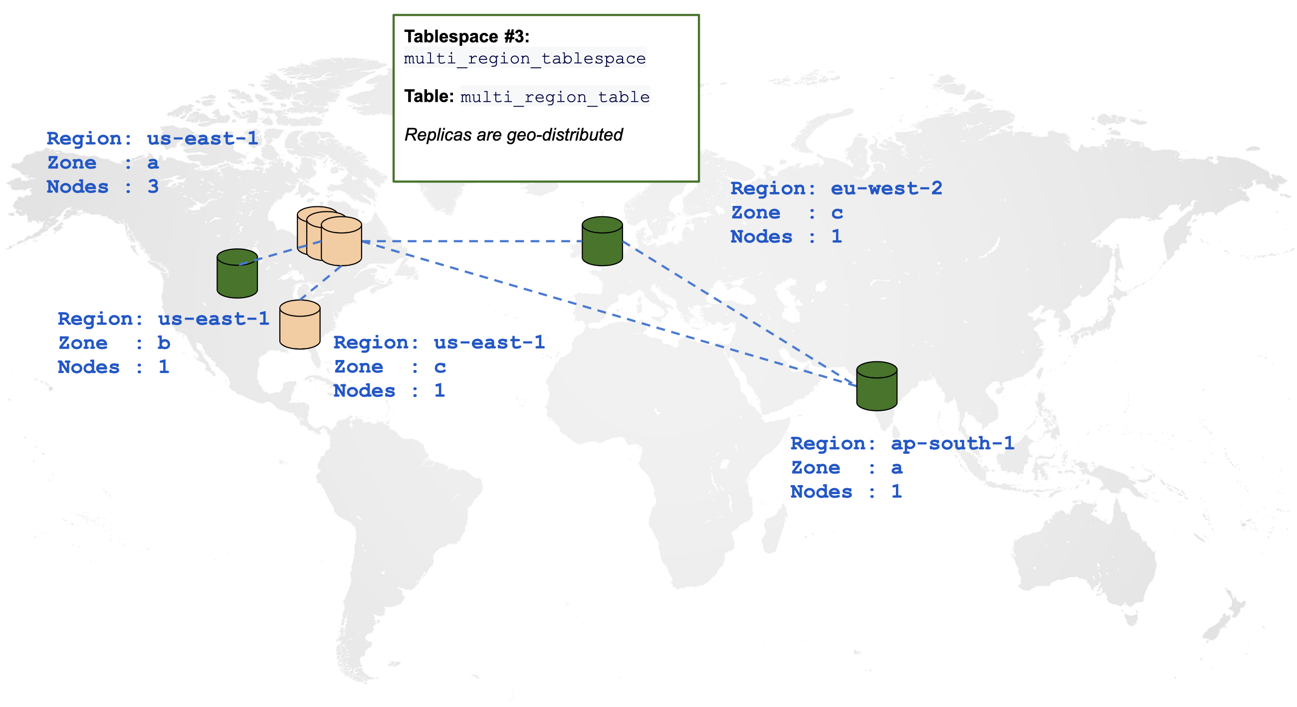
The following diagram is a graphical representation of a table spread across multiple regions:
CREATE TABLESPACE multi_region_tablespace
  WITH (replica_placement='{"num_replicas": 3, "placement_blocks": [
    {"cloud":"aws","region":"us-east-1","zone":"us-east-1b","min_num_replicas":1},
    {"cloud":"aws","region":"ap-south-1","zone":"ap-south-1a","min_num_replicas":1},
    {"cloud":"aws","region":"eu-west-2","zone":"eu-west-2c","min_num_replicas":1}]}');

CREATE TABLE multi_region_table (id INTEGER, field text)
  TABLESPACE multi_region_tablespace SPLIT INTO 1 TABLETS;
The following demonstrates how to measure the latencies incurred for INSERTs and SELECTs on this table, where the client is in us-east-1a zone:
yugabyte=# INSERT INTO multi_region_table VALUES (1, 'field1'), (2, 'field2'), (3, 'field3');
Time: 863.616 ms
yugabyte=# SELECT * FROM multi_region_table;
 id | field
----+--------
  3 | field3
  2 | field2
  1 | field1
(3 rows)

Time: 337.154 ms
Leader preference
Leader preference helps optimize workloads that require distribution of data over multiple zones for zone-level fault tolerance, but which have clients only in a subset of those zones. It overrides the default behavior of spreading the tablet leaders across all placement zones of the tablespace, and instead places them closer to the clients.
The leaders handle all reads and writes, which reduces the number of network hops, which in turn reduces latency for increased performance. Leader preference allows you to specify the zones in which to place the leaders when the system is stable, and fallback zones when an outage or maintenance occurs in the preferred zones.
In the following example our tablespace is setup to have replicas in us-east-1, us-east-2 and us-west-1. This enables it to survive the loss of an entire region. The clients are located in us-east-1. By default we would have a third of the leaders in us-west-1, which has a latency of 62ms from our clients.
CREATE TABLESPACE us_east1_region_tablespace
  WITH (replica_placement='{"num_replicas": 3, "placement_blocks": [
    {"cloud":"aws","region":"us-east-1","zone":"us-east-1b","min_num_replicas":1,"leader_preference":1},
    {"cloud":"aws","region":"us-east-2","zone":"us-east-2a","min_num_replicas":1,"leader_preference":2},
    {"cloud":"aws","region":"us-west-1","zone":"us-west-1a","min_num_replicas":1}]}');

CREATE TABLE preferred_leader_table (id INTEGER, field text)
  TABLESPACE us_east1_region_tablespace;
yugabyte=# INSERT INTO preferred_leader_table VALUES (1, 'field1'), (2, 'field2'), (3, 'field3');
Time: 43.712 ms
yugabyte=# SELECT * FROM preferred_leader_table;
 id | field
----+--------
  3 | field3
  2 | field2
  1 | field1
(3 rows)

Time: 1.052 ms
Setting leader_preference of us-east-1b to 1 (most preferred) informs the YugabyteDB load balancer to place all associated tablet leaders in this zone, dropping the latency to less than 1ms. If all the nodes in us-east-1a are unavailable, they we will fallback to the next preferred zone us-east2 which only has a 12ms latency.
You can specify non-zero contiguous integer values for each zone. When multiple zones have the same preference, the leaders will be evenly spread across them. Zones without any values are least preferred.
You can check the overall leader distribution and cluster level leader preference on the tablet-servers page.
Indexes
Like tables, indexes can be associated with a tablespace. If a table has more than one index, YugabyteDB picks the closest index to serve the query. The following example creates three indexes for each region occupied by the multi_region_table from above:
CREATE TABLESPACE us_east_tablespace
  WITH (replica_placement='{"num_replicas": 1, "placement_blocks": [
    {"cloud":"aws","region":"us-east-1","zone":"us-east-1b","min_num_replicas":1}]}');

CREATE TABLESPACE ap_south_tablespace
  WITH (replica_placement='{"num_replicas": 1, "placement_blocks": [
    {"cloud":"aws","region":"ap-south-1","zone":"ap-south-1a","min_num_replicas":1}]}');

CREATE TABLESPACE eu_west_tablespace
  WITH (replica_placement='{"num_replicas": 1, "placement_blocks": [
    {"cloud":"aws","region":"eu-west-2","zone":"eu-west-2c","min_num_replicas":1}]}');

CREATE INDEX us_east_idx ON multi_region_table(id) INCLUDE (field) TABLESPACE us_east_tablespace;
CREATE INDEX ap_south_idx ON multi_region_table(id) INCLUDE (field) TABLESPACE ap_south_tablespace;
CREATE INDEX eu_west_idx ON multi_region_table(id) INCLUDE (field) TABLESPACE eu_west_tablespace;
Now run the following EXPLAIN command by connecting to each region:
EXPLAIN SELECT * FROM multi_region_table WHERE id=3;
EXPLAIN output for querying the table from us-east-1:
                                         QUERY PLAN
---------------------------------------------------------------------------------------------
 Index Only Scan using us_east_idx on multi_region_table  (cost=0.00..5.06 rows=10 width=36)
   Index Cond: (id = 3)
(2 rows)
EXPLAIN output for querying the table from ap-south-1:
                                          QUERY PLAN
----------------------------------------------------------------------------------------------
 Index Only Scan using ap_south_idx on multi_region_table  (cost=0.00..5.06 rows=10 width=36)
   Index Cond: (id = 3)
(2 rows)
EXPLAIN output for querying the table from eu-west-2:
                                         QUERY PLAN
---------------------------------------------------------------------------------------------
 Index Only Scan using eu_west_idx on multi_region_table  (cost=0.00..5.06 rows=10 width=36)
   Index Cond: (id = 3)
(2 rows)
What's Next?
The following features will be supported in upcoming releases:
- Using
ALTER TABLEto change theTABLESPACEspecified for a table. - Support
ALTER TABLESPACE. - Setting read replica placements using tablespaces.
- Setting tablespaces for colocated tables and databases.
Conclusion
YSQL Tablespaces thus allow specifying placement policy on a per-table basis. The ability to control the placement of tables in a fine-grained manner provides the following advantages:
- Tables with critical information can have higher replication factor and increased fault tolerance compared to the rest of the data.
- Based on the access pattern, a table can be constrained to the region or zone where it is more heavily accessed.
- A table can have an index with an entirely different placement policy, thus boosting the read performance without affecting the placement policy of the table itself.
- Coupled with Table Partitioning, tablespaces can be used to implement Row-Level Geo-Partitioning. This allows pinning the rows of a table in different geo-locations based on the values of certain columns in that row.